Thermocouples - The Basics

Contents

1. Thermocouple Basic Principle
2. Calibration and Non-Linearity
3. Cold Junction Compensation
4. Thermocouple Material Types
5. Summary

Thermocouple Basic Principle

When a temperature gradient exists along a conductor, electrons flow, generating a voltage (EMF). This phenomenon—discovered by Thomas Seebeck in 1822—is the basis for thermocouple operation. The magnitude and direction of the EMF depend on both the temperature gradient and the material's properties.

However, a single homogeneous conductor produces no measurable voltage in a closed circuit because the internal EMFs cancel out. To generate a usable signal, two dissimilar conductors (materials A and B) are joined, forming a thermocouple. When exposed to a temperature gradient (Figure 2.1), these materials respond differently, creating a net EMF (Figure 2.2).

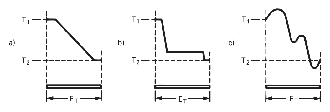
Figures 2.1 a,b,c: Temperature Distributions Resulting in Same Thermoelectric EMF


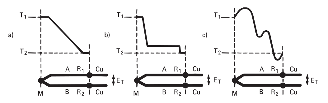
Figures 2.2 a,b,c: Thermocouple EMFs Generated by Temperature Gradients

i Key Point: The EMF is generated not at the junction itself, but along the conductor where the temperature gradient exists. Therefore:

• Conductors must be chemically and physically uniform where gradients occur.
• Junctions must be in isothermal (constant temperature) zones to avoid unwanted EMFs.

As long as the conductors are homogeneous, the EMF generated between temperatures T1 and T2 will be the same, regardless of how the gradient is distributed (see Figure 2.2 again). The thermocouple’s output is determined solely by the temperatures at:

• M: the measuring junction
• R: the reference junction (where dissimilar wires connect to copper)

The reference junction must be held at a known, stable temperature—this is why thermocouples are differential, not absolute, temperature sensors.

Calibration and Non-Linearity

Thermocouples don’t produce a linear voltage-to-temperature output. The relationship varies across temperature ranges and materials. This is why calibration tables are essential—they link thermocouple voltage to corresponding temperatures.

Figure 2.3 shows how Seebeck coefficients (voltage sensitivity) vary for different thermocouple types. For accurate temperature readings, thermocouple voltages must be interpreted using these calibration curves or converted using interpolation and signal processing electronics.

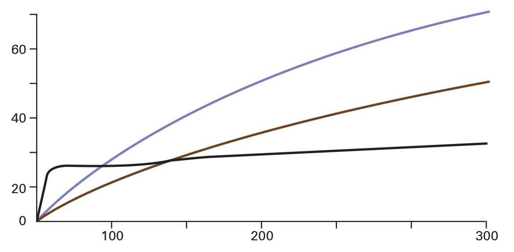
Figure 2.3: Seebeck coefficients for Types E, T and Nickel Chromium vs. Au - 0.07% Fe thermocouples

Cold Junction Compensation

Calibration tables assume the reference junction is at 0°C. But in real-world conditions, this isn’t always possible. So we use cold junction compensation.

Traditionally, reference junctions could be placed in melting ice or temperature-controlled blocks. Nowadays, compensation is done electronically—typically with a thermistor or similar sensor located near the reference junction. This device senses the actual temperature and corrects the thermocouple reading automatically.

i Linearisation and compensation electronics are now standard in most industrial systems, ensuring accuracy across a wide temperature range and correcting for non-linearity.

Thermocouple Material Types

While many conductors exhibit thermoelectric effects, only a few are suitable for practical temperature measurement. Key considerations include:

• Signal strength
• Linearity
• Stability over time and temperature
• Repeatability

Over decades, specific combinations of metals and alloys have been standardised into internationally recognised types (e.g., Types K, J, T, E, N, R, S, and B), defined by standards like BS EN 60584-1 and IEC 60584.

Thermocouples are broadly grouped into:

• Base metal types (e.g., K, J, T): Cheaper, with higher signal outputs. Typical range: 0–1,200°C.
• Noble/rare metal types (e.g., R, S, B): More stable and accurate, but more expensive. Typical range: ambient to 2,000°C plus.

⚠️ Note on Type K: While widely used, Type K can show instability at high temperatures or over long periods. Type N (Nicrosil/Nisil) was developed as an alternative, offering improved stability and extended temperature range, while retaining base-metal affordability.

Summary

Thermocouples work by generating an electromotive force (EMF) in response to a temperature gradient, with the output voltage depending on the gradient and the materials used. This effect, discovered by Seebeck in 1822, is the basis of thermocouple sensors, which require two dissimilar materials to generate a usable voltage. The output is influenced by the temperature of the measuring and reference junctions, with the reference junction typically kept at a constant temperature. Calibration tables are needed for accurate temperature measurements due to the non-linear nature of thermocouple voltage outputs. Cold junction compensation, often done with electronics or by placing the reference junction in a controlled environment, corrects for variations in reference junction temperature. Thermocouple materials are chosen based on factors like temperature range, signal strength, and repeatability, with rare metal types offering better stability at higher costs, while base metal types are cheaper but less stable.

Further Reading

What are the various thermocouple types?
Explore the features and characteristics of the various thermocouple types

Thermocouple Output Tables
View EMF versus Temperature tables for all thermocouple types.

What are the thermocouple colour codes?
Explore thermocouple colour codes for cable and connectors.